TF-Notes

Shallow Neural Networks v.s. Deep Neural Networks

Shallow Neural Networks:

• Consist of one hidden layer (occasionally two, but rarely more).
• Typically take inputs as feature vectors, where preprocessing transforms raw data into structured inputs.

Deep Neural Networks:

• Consist of three or more hidden layers.
• Handle larger numbers of neurons per layer depending on model design.
• Can process raw, high-dimensional data such as images, text, and audio directly, often using specialized architectures like Convolutional Neural Networks (CNNs) for images or Recurrent Neural Networks (RNNs) for sequences.

Why deep learning took off: Advancements in the field

• ReLU Activation Function:
  • Solves the vanishing gradient problem, enabling the training of much deeper networks.
• Availability of More Data:
  • Deep learning benefits from large datasets which have become accessible due to the growth of the internet, digital media, and data collection tools.
• Increased Computational Power:
  • GPUs and specialized hardware (e.g., TPUs) allow faster training of deep models.
  • What once took days or weeks can now be trained in hours or days.
• Algorithmic Innovations:
  • Advancements such as batch normalization, dropout, and better weight initialization have improved the stability and efficiency of training.
• Plateau of Conventional Machine Learning Algorithms:
  • Traditional algorithms often fail to improve after a certain data or model complexity threshold.
  • Deep learning continues to scale with data size, improving performance as more data becomes available.

In short:

The success of deep learning is due to advancements in the field, the availability of large datasets, and powerful computation.

CNNs (supervised tasks) vs. Traditional Neural Networks:

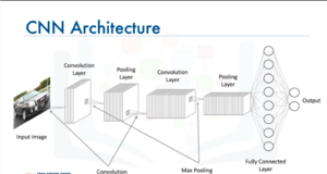
• CNNs are considered deep neural networks. They are specialized architectures designed for tasks involving grid-like data, such as images and videos. Unlike traditional fully connected networks, CNNs utilize convolutions to detect spatial hierarchies in data. This enables them to efficiently capture patterns and relationships, making them better suited for image and visual data processing. Key Features of CNNs:
  • Input as Images: CNNs directly take images as input, which allows them to process raw pixel data without extensive manual feature engineering.
  • Efficiency in Training: By leveraging properties such as local receptive fields, parameter sharing, and spatial hierarchies, CNNs make the training process computationally efficient compared to fully connected networks.
  • Applications: CNNs excel at solving problems in image recognition, object detection, segmentation, and other computer vision tasks.

Convolutional Layers and ReLU

• Convolutional Layers apply a filter (kernel) over the input data to extract features such as edges, textures, or patterns.
• After the convolution operation, the resulting feature map undergoes a non-linear activation function, commonly ReLU (Rectified Linear Unit).

Pooling Layers

Pooling layers are used to down-sample the feature map, reducing its size while retaining important features.

Why Use Pooling?

• Reduces dimensionality, decreasing computation and preventing overfitting.
• Keeps the most significant information from the feature map.
• Increases the spatial invariance of the network (i.e., the ability to recognize patterns regardless of location).

Keras Code

One Set of Convolutional and Pooling Layers:

model = Sequential()

model.add(Input(shape=(28, 28, 1)))

model.add(Conv2D(16, (5, 5), strides=(1, 1), activation='relu'))

model.add(MaxPooling2D(pool_size=(2, 2), strides=(2, 2)))

   

model.add(Flatten())

model.add(Dense(100, activation='relu'))

model.add(Dense(num_classes, activation='softmax'))

   

    # compile model

model.compile(optimizer='adam', loss='categorical_crossentropy',  metrics=['accuracy'])

Two Sets of Convolutional and Pooling Layers:

model = Sequential()

model.add(Input(shape=(28, 28, 1)))

model.add(Conv2D(16, (5, 5), activation='relu'))

model.add(MaxPooling2D(pool_size=(2, 2), strides=(2, 2)))

   

model.add(Conv2D(8, (2, 2), activation='relu'))

model.add(MaxPooling2D(pool_size=(2, 2), strides=(2, 2)))

   

model.add(Flatten())

model.add(Dense(100, activation='relu'))

model.add(Dense(num_classes, activation='softmax'))   

# Compile model

model.compile(optimizer='adam', loss='categorical_crossentropy',  metrics=['accuracy'])

Recurrent Neural Networks (supervised tasks)

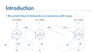
• Recurrent Neural Networks (RNNs) are a class of neural networks specifically designed to handle sequential data. They have loops that allow information to persist, meaning they don't just take the current input at each time step but also consider the output (or hidden state) from the previous time step. This enables them to process data where the order and context of inputs matter, such as time series, text, or audio.

How RNNs Work:

1. 
   Sequential Data Processing:
   • At each time step t, the network takes:
     • The current input xt​,
     • A bias bt​,
     • And the hidden state (output) from the previous time step, at−1​.
   • These are combined to compute the current hidden state at​.
2. Recurrent Connection:
   • The feedback loop, as shown in the diagram, allows information to persist across time steps. This is the "memory" mechanism of RNNs.
   • The connection between at−1​ (previous state) and zt​ (current computation) captures temporal dependencies in sequential data.
3. Activation Function:
   • The raw output zt​ passes through a non-linear activation function f (commonly tanh or ReLU) to compute at​, the current output or hidden state.

Long Short-Term Memory (LSTM) Model

Popular RNN variant (LSTM for short)

LSTMs are a type of Recurrent Neural Network (RNN) that solve the vanishing gradient problem, allowing them to capture long-term dependencies in sequential data. They achieve this through a memory cell and a system of gates that regulate the flow of information.

---

Applications Include:

1. Image Generation:
   • LSTMs generate images pixel by pixel or feature by feature.
   • Often combined with Convolutional Neural Networks (CNNs) for spatial feature extraction.
2. Handwriting Generation:
   • Learn sequences of strokes and predict future strokes to generate realistic handwriting.
   • Can mimic human writing styles given text input.
3. Automatic Captioning for Images and Videos:
   • Combines CNNs (for extracting visual features) with LSTMs (for generating captions).
   • Example: "A group of people playing soccer in a field."

---

Key Features of LSTMs

1. Memory Cell:
   • Stores information for long durations, addressing the short-term memory limitations of standard RNNs.
2. Gating Mechanism:
   • Forget Gate: Decides which parts of the memory to discard.
   • Input Gate: Determines what new information to add to the memory.
   • Output Gate: Controls what part of the memory is output at the current step.
3. Handles Long-Term Dependencies:
   • LSTMs can maintain context over hundreds of time steps, making them suitable for tasks like text generation, speech synthesis, and video processing.
4. Flexible Sequence Modeling:
   • Suitable for variable-length input sequences, such as sentences, time-series data, or video frames.

---

Additional Notes

• Variants:
  • GRUs (Gated Recurrent Units): A simplified version of LSTMs with fewer parameters, often faster to train but sometimes less effective for longer dependencies.
  • Bi-directional LSTMs: Process sequences in both forward and backward directions, capturing past and future context simultaneously.
• Use Cases Beyond the Above:
  • Speech Recognition: Transcribe spoken words into text.
  • Music Generation: Compose music by predicting the sequence of notes.
  • Anomaly Detection: Detect unusual patterns in time-series data, like network intrusion or equipment failure.
• Challenges:
  • LSTMs are computationally more expensive compared to simpler RNNs.
  • They require careful hyperparameter tuning (e.g., learning rate, number of layers, units per layer).

Autoencoders (unsupervised learning)

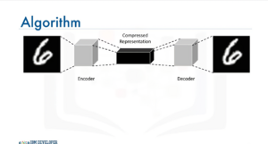
Autoencoding is a type of data compression algorithm where the compression (encoding) and decompression (decoding) functions are learned automatically from the data, typically using neural networks.

Key Features of Autoencoders

1. Unsupervised Learning:
   • Autoencoders are unsupervised neural network models.
   • They use backpropagation, but the input itself acts as the output label during training.
2. Data-Specific:
   • Autoencoders are specialized for the type of data they are trained on and may not generalize well to data that is significantly different.
3. Nonlinear Transformations:
   • Autoencoders can learn nonlinear representations, which makes them more powerful than techniques like Principal Component Analysis (PCA) that can only handle linear transformations.
4. Applications:
   • Data Denoising: Removing noise from images, audio, or other data.
   • Dimensionality Reduction: Reducing the number of features in data while preserving key information, often used for visualization or preprocessing.

Types of Autoencoders

• Standard Autoencoders:
  • Composed of an encoder-decoder structure with a bottleneck layer for compressed representation.
• Denoising Autoencoders:
  • Designed to reconstruct clean data from noisy inputs.
• Variational Autoencoders (VAEs):
  • A probabilistic extension of autoencoders that can generate new data points similar to the training data.
• Sparse Autoencoders:
  • Include a sparsity constraint to learn compressed representations efficiently.

Clarifications on Specific Points

1. Restricted Boltzmann Machines (RBMs):
   • While RBMs are related to autoencoders, they are not the same.
   • RBMs are generative models used for pretraining deep networks, and they are not autoencoders.
   • A more closely related concept is Deep Belief Networks (DBNs), which combine stacked RBMs.
2. Fixing Imbalanced Datasets:
   • While autoencoders can be used to oversample minority classes by learning the structure of the minority class and generating synthetic samples, this is not their primary application.

Applications of Autoencoders

1. Data Denoising:
   • Remove noise from images, audio, or other forms of data.
2. Dimensionality Reduction:
   • Learn compressed representations for data visualization or feature extraction.
3. Estimating Missing Values:
   • Reconstruct missing data by leveraging patterns in the dataset.
4. Automatic Feature Extraction:
   • Extract meaningful features from unstructured data like text, images, or time-series data.
5. Anomaly Detection:
   • Learn normal patterns in the data and identify deviations, useful for fraud detection, network intrusion, or manufacturing defect identification.
6. Data Generation:
   • Variational autoencoders can generate new, similar data points, such as synthetic images.

Keras Advanced Features

• Sequential API: Used for simple, linear stacks of layers.
• Functional API: Designed for more flexibility and control, enabling the creation of intricate models such as:
  • Models with multiple inputs and outputs.
  • Shared layers that can be reused.
  • Models with non-sequential data flows, like multi-branch or residual networks.

---

Advantages of the Functional API:

1. Flexibility: Enables construction of complex architectures like multi-branch and hierarchical models.
2. Clarity: Provides an explicit and clear representation of the model structure.
3. Reusability: Layers or models can be reused across different parts of the architecture.

---

Real-World Applications:

1. Healthcare:
   • Medical image analysis for disease detection (e.g., pneumonia detection from chest X-rays).
2. Finance:
   • Predicting market trends using time-series data.
3. Autonomous Driving:
   • Object detection for pedestrians or vehicles.
   • Lane detection for road safety systems.

Keras Functional API and Subclassing API

from tensorflow.keras.models import Model

from tensorflow.keras.layers import Input, Dense

1. Define the input

inputs = Input(shape=(784,))

1. Define the layers

x = Dense(64, activation='relu')(inputs)

outputs = Dense(10, activation='softmax')(x)

1. Create the model

model = Model(inputs=inputs, outputs=outputs)

model.summary()

Handling multiple inputs and outputs

from tensorflow.keras.models import Model

from tensorflow.keras.layers import Input, Dense, concatenate

# Define two sets of inputs

inputA = Input(shape=(64,))

inputB = Input(shape=(128,))

# The first branch operates on the first input

x = Dense(8, activation='relu')(inputA)

x = Dense(4, activation='relu')(x)

# The second branch operates on the second input

y = Dense(16, activation='relu')(inputB)

y = Dense(4, activation='relu')(y)

# Combine the outputs of the two branches

combined = concatenate([x, y])

# Add fully connected (FC) layers and a regression output

z = Dense(2, activation='relu')(combined)

z = Dense(1, activation='linear')(z)

# Create the model

model = Model(inputs=[inputA, inputB], outputs=z)

model.summary()

Shared layers and complex architectures

from tensorflow.keras.models import Model

from tensorflow.keras.layers import Input, Dense, Lambda

# Define the input layer

input = Input(shape=(28, 28, 1))

# Define a shared convolutional base

conv_base = Dense(64, activation='relu')

# Process the input through the shared layer

processed_1 = conv_base(input)

processed_2 = conv_base(input)

# Create a model using the shared layer

model = Model(inputs=input, outputs=[processed_1,processed_2])

model.summary()

Practical example: Implementing a complex model

from tensorflow.keras.models import Model

from tensorflow.keras.layers import Input, Dense, Lambda, Conv2D, MaxPooling2D, Flatten

from tensorflow.keras.activations import relu, linear

# First input model

inputA = Input(shape=(32, 32, 1))

x = Conv2D(32, (3, 3), activation=relu)(inputA)

x = MaxPooling2D((2, 2))(x)

x = Flatten()(x)

x = Model(inputs=inputA, outputs=x)

# Second input model

inputB = Input(shape=(32, 32, 1))

y = Conv2D(32, (3, 3), activation=relu)(inputB)

y = MaxPooling2D((2, 2))(y)

y = Flatten()(y)

y = Model(inputs=inputB, outputs=y)

# Combine the outputs of the two branches

combined = concatenate([x.output, y.output])

# Add fully connected (FC) layers and a regression output

z = Dense(64, activation='relu')(combined)

z = Dense(1, activation='linear')(z)

# Create the model

model = Model(inputs=[x.input, y.input], outputs=z)

model.summary()

Keras subclassing API

• Offers flexibility
• Defines custom and dynamic models
• Implements subclassing of the model class and call method
• Used in research and development for sturom training loops and non standard architectures.

import tensorflow as tf

# Define your model by subclassing

class MyModel(tf.keras.Model):

def __init__(self):

super(MyModel, self).__init__()

# Define layers

self.dense1 = tf.keras.layers.Dense(64, activation='relu')

self.dense2 = tf.keras.layers.Dense(10, activation='softmax')

def call(self, inputs):

# Forward pass

x = self.dense1(inputs)

y = self.dense2(x)

return y

# Instantiate the model

model = MyModel()

model.summary()

# Define loss function

loss_fn = tf.keras.losses.SparseCategoricalCrossentropy()

optimizer = tf.keras.optimizers.Adam()

# Compile the model

model.compile(optimizer=optimizer, loss=loss_fn, metrics=['accuracy'])

Use Cases for the Keras Subclassing API:

1. Models with Dynamic Architecture:
   • The Subclassing API is ideal for creating models with architectures that vary dynamically based on the input or intermediate computations.
   • Example: Recurrent neural networks (RNNs) with variable sequence lengths or architectures that depend on runtime conditions.
2. Custom Training Loops:
   • The Subclassing API offers fine-grained control over the training process, allowing you to implement custom training loops using GradientTape.
   • Example: Adversarial training (e.g., GANs) or reinforcement learning models where standard .fit() may not suffice.
3. Research and Prototyping:
   • It is particularly suited for rapid experimentation in research scenarios, enabling you to define and test novel model architectures.
   • Example: Exploring new layer types, loss functions, or combining multiple types of inputs and outputs.
4. Dynamic Graphs:
   • The Subclassing API allows you to implement eager execution with dynamic computation graphs, offering flexibility to perform different operations at each step of the forward pass.
   • Example: Models that use conditional logic or operations like if/else during the forward pass, such as graph neural networks or decision-tree-inspired neural networks.

Dropout Layers

Dropout is a regularization technique that randomly zeroes out a fraction of neuron outputs during each training step. This reduces the network’s reliance on specific neurons and fosters more robust feature learning—helping mitigate overfitting.

Training vs. Inference

• Dropout is active only during training, where it stochastically drops neurons.
• At inference (testing/prediction), dropout is effectively disabled (or rescaled to preserve expected outputs).

Dropout Rate (Hyperparameter)

• Determines the probability of zeroing out each neuron’s output.
• Common values range from 0.2 to 0.5, but it’s dataset and architecture dependent.

TensorFlow Keras Example

from tensorflow.keras.layers import Dropout

# Apply 50% dropout

dropout_layer = Dropout(rate=0.5)(hidden_layer)

Overall, dropout promotes generalization by preventing co-adaptation of neurons. It is an easy-to-use, widely adopted method for combating overfitting in deep networks.

Summary

• Dropout randomly “turns off” neurons during training.
• It is disabled at inference, ensuring consistent outputs.
• The dropout rate sets the fraction of neurons dropped (typical ranges: 0.2–0.5).
• TensorFlow (and other frameworks) make it straightforward to implement.

Batch Normalization

Batch Normalization (BatchNorm) stabilizes and accelerates neural network training by normalizing activations across the current mini-batch. This reduces internal covariate shift—i.e., shifts in input distributions over time—and often enables using larger learning rates for faster convergence.

• Operation
  • Normalizes each channel to have near-zero mean and unit variance (based on the current mini-batch statistics).
  • During training, BatchNorm uses batch statistics; during inference, it uses running averages of mean and variance.
• Learnable Scale & Shift
  • Each BatchNorm layer introduces two trainable parameters: γ (scale) and β (shift). These parameters allow the model to adjust or “undo” normalization if needed, preserving representational power.

• TensorFlow Keras Example

from tensorflow.keras.layers import BatchNormalization

batch_norm_layer = BatchNormalization()(hidden_layer)

Overall, BatchNorm often yields faster training, improved stability, and can help networks converge in fewer epochs.

• Summary
  • BatchNorm normalizes activations, reducing internal covariate shift.
  • It’s used both in training (via batch statistics) and inference (via running averages).
  • Introduces two learnable parameters for scaling and shifting post-normalization.
  • Can allow higher learning rates and faster convergence.

Keras Custom Layers

Custom layers allow the developer to:

• Implement novel research ideas using:
  • New algorithms or techniques
• Optimize performance to suit
  • Specific data
  • Computational constraints
• Enhance flexibility by defining
  • Unique behaviors
• Improve readability and maintenance by
  • Reusable components